Data teams are increasingly looking for ways to unify data modeling and governance within a single, scalable platform. Databricks has cemented its position in the market with a powerful lakehouse architecture that blends data engineering, data science, and analytics capabilities.
Read our "Hands-on Databricks" Blog-Series: |
| 1. How to leverage SAP Databricks to integrate ServiceNow Data |
| 2. Data Modeling with dbt on Databricks: A Practical Guide |
| 3. Databricks AutoML for Time-Series: Fast, Reliable Sales Forecasting |
| 4. Advanced Data Warehousing in Databricks with DBT Macros and Snapshots |
Unlike traditional Data Warehouse software, sold as a finished application by vendors like SAP or Oracle, Databricks is a platform on which you can build a SQL-based warehouse. To achieve this, a team would have to choose and adapt a warehousing design pattern and logical framework to build their logical data model in.
The open source data transformation tool dbt (data build tool) has become the industry standard framework for SQL-first transformations and data modeling. It is a perfect fit for building an Enterprise Data Warehouse on Databricks.
Bringing these two together allows analysts and engineers to transform raw data into reliable, production-ready datasets directly on the Databricks platform using best practices from software engineering. With the release of dbt support in Databricks Jobs, you can fully utilize the power of Databricks to run, orchestrate and monitor your dbt workflows directly within the platform.

In this blog post, we demonstrate how to combine dbt and Databricks to create scalable, reliable and performant data transformations based on an example workflow for data warehousing: bringing in data from various source systems and refining information in a Medallion architecture for analysis and reuse. We will walk you through the necessary steps:
- Creating a skeleton dbt project and bringing it to Databricks via a Git repository
- Defining the intended stages of data modeling using dbt
- Setting up a Databricks compute cluster to run the dbt project
- Configuring a Databricks Job to execute the dbt project stages
Finally, we will take a look at how dbt can help handle changing data points over time and changing data schema.
Project Setup: Local Initialization and Project Transport
Before you can run dbt jobs in Databricks, you’ll need to initialize a dbt project and configure it to connect to your Databricks workspace. The most common workflow sees you initializing the dbt project locally and then deploying it on Databricks using the Workspaces Git integration.
Initialize dbt locally
Start by creating your project in a local development environment. Using the dbt-databricks adapter, you can scaffold a new project with:
pip install dbt-core dbt-databricks
dbt init my_dbt_project
1. Create dbt project root
During setup, choose Databricks as your target adapter. You will be asked to provide connection information for your databricks instance, as well as a Databricks Access Token. After the process is finished, it will create the standard dbt directory structure (models/, seeds/, tests/, etc.) and a dbt_project.yml configuration file.

2. Transport the project to Databricks
Once the project is working locally, the next step is to make it accessible inside Databricks. The recommended approach is to push your dbt project into a Git repository, then link that repository to your Databricks workspaceRepos. Git ensures strict version control on the code base, manages multi-user collaboration and conflict resolution, and can be used to determine exactly which version of the workflow to run in the production environment.

Watch the recording of our Webinar: "Bridging Business and Analytics: The Plug-and-Play Future of Data Platforms"
Data modeling with dbt
At this point, you’ve got the skeletonbones dbt project that can run locally for development, and is now available in your Databricks environment for production-ready execution. The next steps are to implement your data model and then create the Databricks Job to orchestrate dbt runs, where your transformations can be scheduled, monitored, and scaled automatically.
Let’s start with the data model: In our use case, we want to implement the commonly used medallion architecture, a design pattern popularized by Databricks. Here data is structured in three layers, Bronze (raw data), Silver (cleaned & structured data) and Gold (enriched data), with every step progressively combining data with the goal of creating metrics and extracting business insights for reporting purposes.
To simulate the interconnectedness of data landscapes in modern business use cases, our data sources for this example originate from multiple data sources as well. One table is extracted from a postgreSQL database that is connected to the Databricks Unity Catalog via Lakehouse Federation. The other is a delta table saved in our Databricks Catalog directly.
Bronze Layer: Persisting data from all sources
The first step of implementing the medallion architecture is to clone the raw data to our bronze level tables. This is done to collect all data in the same system, at the same place. Keep in mind that at this stage, no logical transformations nor enrichments of data are being done.
This is where the dbt models come into play. There, data sources as well as the targets, including any transformations are being defined. This is done via the sources.yml file in the /models directory as well as .sql-files in the dbt models folder structure. This is also where you can hierarchically structure your data model according to your needs.

In our case, the two sources are being defined in the sources.yml file like this:
version: 2
sources:
  - name: sap_erp_file_export
    database: nextlytics
    schema: nextlytics-demo
    tables:
      - name: raw_planvorgaben
  - name: external_postgres
    database: ext_nly_demo_postgres
    schema: public
    tables:
      - name: raw_maschinendaten
This allows dbt to reference those tables by name in the following step and not bother with the technical details of their origin.
For our bronze tables, we just want to clone those sources into delta tables with a specified name. For that, we create a .sql file for each target, with the name of the file specifying the target table to be created.
For example, we want to import all the data from our external postgres table raw_maschinendaten into a table called b_maschinendaten. The prefix b_ signifies that this is in fact a bronze-level table.
Thus we create a file b_maschinendaten.sql with the following contents:

The dbt-tag “bronze” that is included here will become relevant once we get to orchestrating the jobs.
After applying the same logic to our other data source, we end up with the data models for two bronze level tables, b_maschinendaten and b_planvorgaben.
Silver Layer: Refining and cleaning data to reflect business meaning
For our silver layer, we want to combine both of those tables into a single one. Since one of the tables contains information about production machine statistics and the other one holds data for planned machine operations, this data can be joined together neatly using sql.
The sql transformation logic will be applied directly in the model for our silver layer table s_machine_output.
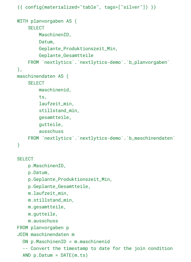
Note that in this example, our Silver layer table still contains German language column names taken more or less directly from the data source. When working with international data teams, applying translations to English is a common best practice for an Enterprise Data Warehouse and should be applied either in Bronze or Silver layer. We will come back to this later to show how dbt can handle such revisions.
Gold Layer: Aggregation and KPI calculation
For our gold layer we want to provide actionable insights for reporting and dashboarding purposes.
Thus we want to calculate essential KPIs derived from the data, in this case we decided to go for OEE (Overall Equipment Effectiveness) to gain insights regarding the effectiveness of our simulated production.
The model for our gold layer table g_oee_performance thus looks like this:
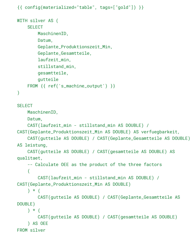
This concludes the data modelling processes we want to execute, the next step is to implement the orchestration using Databricks Jobs.
Preparing Databricks Compute
First some preparatory steps - jobs in Databricks run on Spark clusters. In our case, we need a cluster that fulfills the following requirements:
1. The cluster must have the dbt-databricks python library installed. This can be done via the “Libaries” tab in the Databricks cluster configuration.

2. The cluster must have access to a Databricks Access token to be able to access the Databricks API for the creation of the tables. This can be configured using the cluster's environment variables in combination with the Databricks Secrets management utility.

Configuring and running the Databricks Job
Now that we have the model definitions finished and the cluster prepared, it is time to configure the actual pipeline for the data load and transformation. For this we are going to use the Databricks Jobs interface.
The job we create will in this case be split in three different subtasks for each target layer of the data model, as well as one additional task to generate the SQL to be executed as file output for debugging purposes, in case one of the processing steps might fail.

This is where the tags we set in the model definitions come into play. By assigning those logical groups to processing steps, we are able to execute only a subset of the dbt transformations with a single call. Also take note to select the correct pre-configured cluster for the pipeline execution.

We can now trigger the job via the “Runs” tab. Here we can set up scheduled pipeline executions, check the data lineage and monitor the status of each task/pipeline that has been run.

This concludes the basic setup of how to integrate a dbt data warehousing workflow into Databricks, but there are some more common situations you may find yourself in, that we want to quickly examine here.
Data change tracking and schema changes
Time keeps marching ever onwards and with it, the data output and consumed by your business might change. May it be due to a version update in one of the source systems, a migration to a different source database or new business requirements demanding a shift in your established data structure.
Here we want to take a quick look at how a setup such as this might handle schema evolution (the changing of data structures) and data merges.
Consider that for our silver layer transformation, we want to replace the German column names for more descriptive and unified English translations. In this case we can just slightly alter the SELECT statement in the model definition like this:
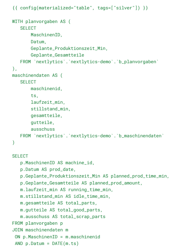
On the next run of the task that updates the Silver layer table, the new column schema will be applied. Now all that is left is to alter the references in the SELECT statement of the gold level table and we’re done.
This works because ❴❴ config(materialized="table") ❵❵ sets the model to do a full table refresh on every data load.
Of course this strategy, while simple to implement, has significant drawbacks when the amount of data increases or schema changes become more common.
For this, dbt offers the option to use incremental models. This allows users to load only new data that has not already been processed via an automatic merge procedure. To do this, you need to provide the configuration ❴❴ config(materialized="incremental") ❵❵ within the model definition.
This opens up a whole new selection of possible approaches, for example you can implement conditional operations within the model’s SELECT statement, that only trigger on an incremental load on an previously existing model. This could look something like this, where a datetime value from the data source is compared to the equivalent from the model table to ascertain whether new data has arrived between pipeline executions:
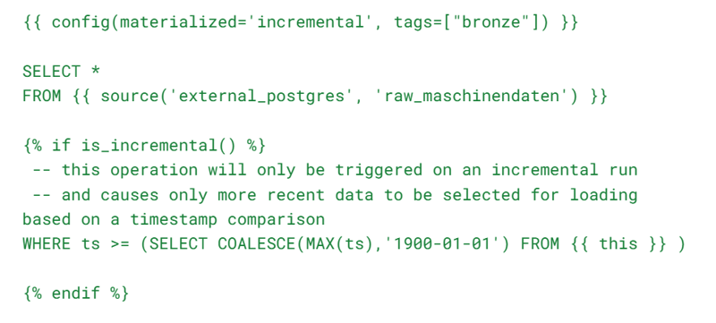
These use cases really only scratch the surface of what is possible by utilizing dbt. There are a myriad of other useful features to handle complex scenarios or performance intensive data loads, that go beyond the scope of this article. Among them are common data warehousing tasks like automatic schema evolution, complexmore granular incremental loading strategies, different merge/deletion scenarios and many more.
From SQL to Enterprise Data Warehouse with dbt: Our Conclusion
Using dbt on Databricks turns a greenfield SQL warehouse into a dependable operating model: a clear Medallion layout, explicit source and model definitions, and reproducible pipelines via Git and Databricks Jobs. Tags let you run targeted subsets, incremental models keep costs in check, and data lineage and monitoring provide transparency from Bronze to Gold layer for business metrics like OEE.
Bottom line: a smooth path from local prototype to production-grade data logistics—versioned, testable, and scalable. If you want to build or modernize your lakehouse with dbt/Databricks, we can help with architecture, implementation, and run-ready operations—practical and to the point.
If you want to know more about how you can use dbt to unlock the full potential of modern data warehousing in Databricks, feel free to contact us!
FAQ - Data modeling with dbt on Databricks
These are some of the most frequently asked questions about data modeling with dbt on Databricks.
Follow any dbt quick start tutorial on the web. In short, you need to follow a few basic steps: pip install dbt-core dbt-databricks → dbt init <project> → choose Databricks adapter, add workspace info + access token; folders like models/, tests/, dbt_project.yml are created.
Push to Git and connect a folder in your Databricks workspace for versioning, team collaboration, and reproducible runs
Using Medallion architecture to build a logical warehouse model is not an exact science but largely up to project and team convention and understanding. Our examples roughly use the following interpretation: Bronze: clone and persist raw data. Silver: clean/standardize & join. Gold: calculate KPIs (e.g., OEE).
Yes, producing a model according to Data Vault specifications is a perfect scenario for using dbt on Databricks. Data Vault logic can be used instead of the Medallion architecture or in synergy with it. Cookie cutter templates for Data Vault modeling with dbt are available, enabling data engineers to quickly build out Hubs, Link and Satellite structures on Databricks.
Use Databricks Jobs: create subtasks per layer, tags to run subsets, schedule/monitor runs, view lineage, and emit SQL artifacts for debugging.
Choose full refresh (simple, costly at scale) or incremental models with is_incremental() and timestamp-based merges for performant growth. Incremental changes in combination with a fully versioned data modeling approach like Data Vault are the gold standard of resilient and reproducible warehousing.
Data Science & Engineering, Databricks

/Logo%202023%20final%20dunkelgrau.png?width=221&height=97&name=Logo%202023%20final%20dunkelgrau.png)


